User’s guide: SLIP

File format

SLIP requires four input files.

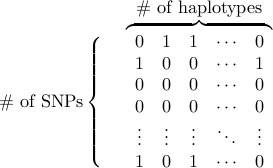
1. Phased reference data file.

: Reference data file is a space-delimitered matrix of 0/1 (0 for major and 1 for minor allele). The allele coded as ‘1’ (minor allele) will be considered the disease allele.
The rows are SNPs and the columns are haplotypes.
Any lines starting with “#” are considred comments in all input files.

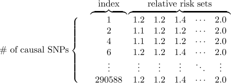
$mbox{# of SNPs} left{ begin{array}{c} end{array} right. overbrace{ begin{array}{ccccc} 0 & 1 & 1 & cdots & 0 1 & 0 & 0 & cdots & 1 0 & 0 & 0 & cdots & 0 0 & 0 & 0 & cdots & 0 vdots & vdots & vdots & ddots & vdots 1 & 0 & 1 & cdots & 0 end {array} }^{mbox{# of haplotypes}}$

2. Causal SNP file.

: Suppose we have SNPs indexed as in reference data.
Causal SNP file determines the subset of the SNPs that we will consider as a putative causal SNP
(possibly after removing too much rare SNPs given a MAF threshold).
The power will be averaged over these causal SNPs.
Each row corresponds to each causal SNP.
The first column is the index of the causal SNP, which is the line number in the reference data (counting starts from 1).
The second column is the relative risk of the putative causal SNP.
You can set a constant relative risk for all causal SNPs, or give higher relative risk for rarer SNPs.
You can specify another set of relative risks using the third column, and yet another set using the fourth column and so on, optionally.
The indexes must be numerically ordered.
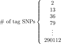
$mbox{# of causal SNPs} left{ begin{array}{c} end{array} right. overbrace{ begin{array}{c} 1246vdots290588 end{array} }^{mbox{index}} overbrace{ begin{array}{ccccc} 1.2 & 1.2 & 1.4 & cdots & 2.0 1.1 & 1.2 & 1.2 & cdots & 2.0 1.1 & 1.2 & 1.2 & cdots & 2.0 1.2 & 1.2 & 1.4 & cdots & 2.0 vdots & vdots & vdots & ddots & vdots 1.2 & 1.2 & 1.4 & cdots & 2.0 end {array} }^{mbox{relative risk sets}}$

3. Tag SNP file.

: This file describes which SNP in the reference data will be genotyped using a certain platform.
Similarly to the causal SNPs, tag SNPs are specified by the index number,
which is the line number of the SNP in the reference data (counting starts from 1).
The indexes must be numerically ordered.

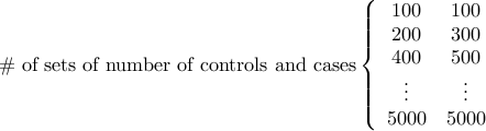
4. Number of individuals file.

: This file describes the numbers of controls and cases that we would like to obtain power estimate.
The first column is the number of controls and the second column is the number of cases.
Each control or case is considered a diploid individual.

Example files

ref.txt.gz (Reference file, 25Mb) 2,605,595 SNPs/ 120 haplotypes/ mimicing the HapMap CEU data
causal.txt.gz (Causal SNP file, 6Mb) 2,234,839 SNPs/ 5 sets of relative risks/ mimicing common SNPs (MAF.05) in the HapMap CEU data
tag.txt.gz (tag SNP file, 1Mb) 420,388 SNPs/ mimicing a 500k chip that overlaps with polymorphic SNPs in the HapMap CEU data
Ns.txt.gz (Number of individuals file, 196b)

Usage

./slip [ref file] [causal file] [tag file] [N file] [prevalance] [permarker thres] [w] [# sampling] [seed]

Parameters
- Reference file (ref file), causal SNP file (causal file), tag SNP file (tag file), and number of individuals file (N file) need to follow the aforementioned format.
- prevalance is the population disease prevalance of the target disease (e.g. 0.1)
- permarker thres is the per-marker significance threshold. This needs to be pre-computed by using SLIDE. Given a SLIP format files, you can easily transform to the SLIDE format by using the format converter described below.
- w is the window size in terms of the number of tag SNPs. For example, if w=100, given a causal SNP, 50 tag SNPs on the left side of the causal SNP and 50 tag SNPs on the right side of the causal SNPs will be used as proxies. (if the causal SNP itself is a tag SNP, 49 tag SNPs on the left, the causal SNP itself, and 50 tag SNPs on the right will be used.)
- # sampling denotes how many times we will sample a causal SNP to get per-causal-SNP power. The power outcome will be the average power over these per-causal-SNP power. A number between 10,000-100,000 can usually be used.
- seed is the seed for the random number generation.
Usage example
- slip ref.txt causal.txt tag.txt Ns.txt 0.1 2.19E-7 100 100000 12345678
Approximate time
- For the example file,~10 m for 100,000 sampling with w=100.
Output
- Standard output as follows.

Example output
#################### Power in percentage (stdev) ######################
#controls #cases          RR_set #1             RR_set #2             RR_set #3
     100           0.00500 (0.00224)     0.00600 (0.00245)     0.02300 (0.00480)
     200           0.02200 (0.00469)     0.02300 (0.00480)     0.12700 (0.01126)
     300           0.04700 (0.00685)     0.04800 (0.00693)     0.52100 (0.02277)
     400           0.11100 (0.01053)     0.11300 (0.01062)     1.37800 (0.03686)
     500           0.24500 (0.01563)     0.25000 (0.01579)     3.05100 (0.05439)
     600           0.45700 (0.02133)     0.47600 (0.02177)     5.70600 (0.07335)
     700           0.74000 (0.02710)     0.77700 (0.02777)     9.45900 (0.09254)
     800           1.20100 (0.03445)     1.25600 (0.03522)    14.04400 (0.10987)
     900           1.77900 (0.04180)     1.87400 (0.04288)    19.06400 (0.12422)
    1000          2.63400 (0.05064)     2.78100 (0.05200)    24.38700 (0.13579)
    1100          3.62200 (0.05908)     3.83000 (0.06069)    29.75300 (0.14457)
    1200          4.91800 (0.06838)     5.18800 (0.07013)    34.66400 (0.15049)
...............
    5000         68.21900 (0.14724)    74.45700 (0.13791)    87.94600 (0.10296)

1st and 2nd column: # of controls and cases specified in the number of individuals files.
3rd and 4th column: power estimate of the tag SNP set for the 1st relative risk set specified in the causal SNP file, and the standard deviation of it. Note that the standard deviation is computed assuming the estimated power is true power, and the stochastic error in the per-marker threshold is not taken into account.
5th and 6th column: power and standard deviation for the 2nd relative risk set, and so on…

Demo

The following figure is the Affymetrix 500K chip’s genome-wide power for the HapMap CEU population, computed by SLIP. SNPs with MAF .05 were considered possible causal SNPs. Disease prevalance of .1 was used. The per-marker threshold of 2.19E-7 corresponding to alpha=.05 is used (computed by SLIDE). Power for 50 different numbers of individuals are evaluated (100/100, …, 5,000/5,000). Power for 5 different relative risks are evaluated as follows.

RR#1: fixed relative risk of 1.2 for all causal SNPs
RR#2: 1.3 for causal SNPs with MAF .1 and 1.2 for others
RR#3: fixed relative risk of 1.3 for all causal SNPs
RR#4: 1.4 for causal SNPs with MAF .1 and 1.3 for others
RR#5: fixed relative risk of 1.4 for all causal SNPs

Given the formatted files and the per-marker threshold computed by SLIDE, it only takes 10 minutes to compute total 250 power estimates using 100,000 sampling and window size of 100. This would have taken a tremendous amount of time if we have used the standard simulation procedure repeatedly constructing case/control panels.

Format converter

SLIP requires the per-marker threshold to be computed in advance. Per-marker threshold takes into account the actual multiple testing burden which is dependent on the correlation structure between tests (between tag SNPs). SLIDE can estimate the per-marker threshold. We provide the converter that transforms SLIP format to SLIDE format. In fact, SLIP format becomes SLIDE format just by taking the rows corresponding to the tag SNPs from the reference file. The converter is included in the SLIP package.

Usage
./slip2slide [ref file] [tag file] [output file]