User’s guide: SLIDE
File format
Data file
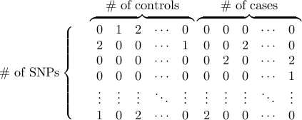
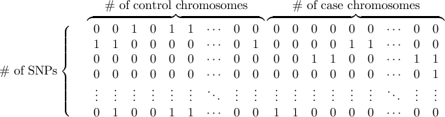
The basic input file is a white-space-delimitered matrix
where 0/1/2 denotes the number of one of two alleles.
The rows are SNPs and the columns are individuals
(controls first, and then cases).
Genotype data or haplotype data can be used.
Any lines starting with “#” are considred comments in all input files.
- Genotype data format
- Haplotype data format
Another possible input file format is the covariance band-matrix.
Let  be the covariance between the statistic at marker
  and
the statistic at marker
and
the statistic at marker  .
(For many cases including the trend test, allelic
.
(For many cases including the trend test, allelic  test, and
Wald test for quantitative traits, turns out to be the correlation coefficient
test, and
Wald test for quantitative traits, turns out to be the correlation coefficient  between
two markers estimated from the dataset.)
Suppose we take into account correlation only when
between
two markers estimated from the dataset.)
Suppose we take into account correlation only when  (e.g. Window size is
  ).
Then, given
).
Then, given  markers indexed as
  ,
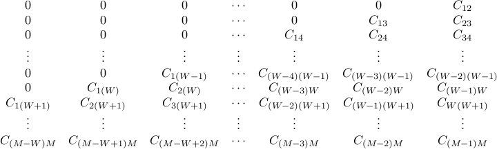
we present the band covariance matrix as the following
,
we present the band covariance matrix as the following 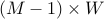 rectangular matrix,
- Band covariance matrix data format
If the genotype or haplotype format is used, SLIDE runs based on the allelic
test or
the Armitage’s trend test respectively for case/control studies,
and based on the Wald test for quantitative traits.Band matrix format allows SLIDE to be applied for a wide variety of statistics, since the user only needs to pre-compute the covariance and provide it.
For example, in our publication, we describe how to compute the covariance for the Weighted haplotype test and the test for imputed genotypes.
Previous studies (Seaman and Muller-Myhsok, AJHG2005) also describe the covariance for other statistics such as the transmission disequilibrium test (TDT).
Note that, if the band matrix format is used, the scaling procedure of SLIDE for higher accuracy will not be used.
In order to maintain the positive semi-definiteness of the correlation matrix, the unknown genotypes need to be resolved beforehand.
The simplest way is to randomly assign missing allele based on the allele frequency. The format converter (PED -> SLIDE) we provide below automatically performs this random asignment.
Another possible way is to assign the allele frequency itself to the allele as a floating point number. Although SLIDE currently does not accept genotype/haplotype format including floating point number, SLIDE accepts the band covariance matrix file, therefore one can compute the covariance based on the assigned floating point number and use it as input to SLIDE.
Yet another possibility is to use available imputation algorithm. After imputation, one can compute the band covariance matrix based on the posterior probabilties of alleles using the derivation described in our publication, and use it as input to SLIDE.
If the number of unknown genotypes is very small compared to the number of known genotypes, the currently implemented approach (random assignment based on frequency) will provide a sufficiently accurate multiple testing correction.
MAP file (optional)
PLINK-format MAP file is optional to display rsid in output.
Example files
- example1.slide.gz (5.4Mb)
Genotype data format/ 5,754 SNPs/ 2,934 controls/ 1,928 cases/ mimicing a chr 22 data of a 500K chip
- example2.slide.gz (230Mb)
Haplotype data format/ 203,689 SNP/ 4,000 control chromosomes/ 4,000 case chromosomes/ mimicing a chr 1 data of 2.7 million HapMap SNPs
- example3.bandcovmat.gz (5.6Mb)
Band covariance matrix format/ 5,754 SNPs/ window size 100
Basic usage
./slide [-G|-H] [data file] [#control] [#case] [w] [tmpdir] [#sampling] [seed] [mapfile(option)]
Parameters
-G is for genotype data and -H is for haplotype data
(Results will be based on the trend test and the test respectively).#control and #case are the numbers of control and case individuals (or chromosomes if -H is used).
w is the window size defined in terms of the number of SNPs.
SLIDE will take into account correlations between SNPs only within this window size (100 is enough for most cases).tmpdir is a temporary storage directory for intermediate files.
#sampling is the number of sampling iterations which can be (roughly) thought of as the number of permutations.
seed is the random number generation seed.
Output
tmpdir/slide.pvalues containing corrected p-values.
Usage example
slide -G example1.slide 2934 1928 100 mydir 10000 12345678
Approximate time
~2 m (example1.slide) and ~1 h (example2.slide) for 10,000 sampling with w=100
Advanced usage
Tests for quantitative traits.
Band covariance matrix input data format.
Utilize a cluster of computer processors.
Split the genome into chromosomes for easier genome-wide analysis.
SLIDE is composed of four programs. (The executable slide for basic usage is nothing more than a wrapper script running these four.)
slide_1prep : data pre-processing.
slide_2run : run the actual sampling.
slide_3sort : sort the maximum statistic.
slide_4correct : correct p-values.
Step 1
./slide_1prep [-G|-H] [data file] [#control] [#case] [w] [prep file]
./slide_1prep [-QG|-QH] [data file] [#individual] [w] [prep file]
./slide_1prep [-C] [band cov mat file] [w] [prep file]
Parameters
Case/control study
-G is for genotype data and -H is for haplotype data
(Results will be based on the trend test and the test respectively).#control and #case are the numbers of control and case individuals (or chromosomes if -H is used).
Quantitative traits
-QG is for genotype data and -QH is for haplotype data
(Results will be based on the Wald test).#individual is the numbers of individuals (or chromosomes if -QH is used).
The trait file is not needed because we make an assumption that the statistic will follow the normal distribution after a random permutation.
w is the window size defined in terms of the number of SNPs.
SLIDE will take into account correlations between SNPs only within this window size (100 is enough for most cases).For band matrix, w has to be the same window size used for constructing the band matrix.
[prep file] is any temporary file name you want to use as a storage file.
Output
Many pre-processed files that look like [prep file].xxxxxx
Usage example
./slide_1prep -G example1.slide 2934 1928 100 mydir/myprepfile
Approximate time
~1 m (example1.slide) and ~0.5 h (example2.slide) with w=100
Step 2
./slide_2run [prep file] [max stat file] [#sampling] [seed]
Parameters
Use the same [prep file] that you specified in step 1.
Output
[max stat file] storing the sampled maximum statistics over the markers.
Usage example
./slide_2run mydir/myprepfile mydir/mymaxstat 10000 12345678
Approximate time
~1 m (example1.slide) and ~0.5 h (example2.slide) with 10,000 sampling and w=100
If you do a large number (e.g. 1,000,000) of sampling, you might want to use a cluster.
Suppose we run 10,000 samplings to create each of 100 max-statistic files,
maxstat1, maxstat2, …, maxstat100,
using 100 CPUs (of course, using different seeds).
Each file only contains binary floats written by the C program.Thus, by merging them as follows,
cat maxstat* > merged_maxstat
we can obtain a merged result file equivalent to 1,000,000 samplings.
If you divide the whole genome into chromosomes, repeat step 1 and step 2 for each chromosome.
Step 3
./slide_3sort [sorted file] [max stat file(chr1)] [max stat file(chr2)] [max stat file(chr3)] ...
Parameters
[max stat file] is the output of step 2.
If you divided genomic region into N independent regions (e.g. chromosomes), provide N max-stat-files. In that case, the number of sampling for each file has to be identical.
If you did not divide the region, just use one max-stat-file.
Output
[sorted file] stores the sorted maximum statistics over the whole genome.
Usage example:
./slide_3sort mydir/mysortedstat mydir/mymaxstat
Step 4
P-value correction
To correct pointwise p-values,
./slide_4correct -p [sorted file] [pointwise-p file] [final output file] [mapfile(optional)]
Parameters
[sorted file] is the output of step 3.
[pointwise-p file] is a text file containing pointwise p-values you want to correct, delimitered by space or newline.
Note that if you used -H or -G option, for each chromosome, step 1 creates a pointwise p-value file which looks like [prep file].txt_pointwisep.
You can use this file to correct p-values of every SNP in each chromosome.You can also specify MAP file to see rsid in output. In that case, the number of SNPs in MAP file has to be the same as the number of pointwise p-values to correct.
Usage example:
./slide_4correct -p mydir/mysortedstat mydir/myprepfile.txt_pointwisep mydir/finaloutput
Output
[final output file] containing corrected p-values, which will look like
#Result based on 10000000 sampling
#SNP_id Pointwise-P     Corrected-P     Approx.STDEV(% of P)    Effective#ofTests       Note
SNP1    1.16801500e-07  4.24000000e-04  6.51014765e-06(1.53541%)        3630
SNP2    2.02511400e-07  7.27500000e-04  8.52625794e-06(1.17199%)        3592
SNP3    3.43213500e-07  1.22440000e-03  1.10584847e-05(0.90318%)        3567
SNP4    5.75063100e-07  2.05320000e-03  1.43142739e-05(0.69717%)        3570
SNP5    9.61198000e-07  3.41440000e-03  1.84465224e-05(0.54026%)        3552
SNP6    1.61919700e-06  5.69580000e-03  2.37978105e-05(0.41781%)        3518
SNP7    2.74274700e-06  9.52860000e-03  3.07210120e-05(0.32241%)        3474
SNP8    4.56832800e-06  1.57566000e-02  3.93806165e-05(0.24993%)        3449
SNP9    7.73045900e-06  2.63954000e-02  5.06938683e-05(0.19206%)        3414
SNP10   1.30862400e-05  4.38772000e-02  6.47703569e-05(0.14762%)        3353
SNP-id will indicate rsid if MAP file is provided.
STDEV is the standard deviation of the corrected p-value estimate, which needs a caution to interpret. If STDEV is very large, then SLIDE’s corrected p-value may not be accurate due to stochastic error. However, even if STDEV is extremely small (e.g.
 ), it does not mean that SLIDE’s corrected p-value
is that extremely near to the true p-value, because SLIDE may converge to a p-value
that differs from the true p-value slightly by 1-2% (which is still accurate).
), it does not mean that SLIDE’s corrected p-value
is that extremely near to the true p-value, because SLIDE may converge to a p-value
that differs from the true p-value slightly by 1-2% (which is still accurate).
If the corrected p-value is extremely close to 1 because the maximum statistic is always more significant than the pointwise p-value, SLIDE just reports the corrected p-value 1 and STDEV 0 (although this can be mathematically misleading, these SNPs are anyhow not of major interest.)
Per-marker threshold estimation
Alternatively, you may want to find the per-marker threshold
for the significance threshold of .05 or .01.
To obtain per-marker thresholds,
./slide_4correct -t [sorted file] [sig threshold file] [final output file]
Parameters
[sig threshold file] is a text file containing significance threshold you want to obtain per-marker threshold, delimitered by space or newline.
Interactive modes
There are interactive modes as well,
./slide_4correct -ip [sorted file] [pointwise-p]
./slide_4correct -it [sorted file] [sig threshold]
Usage example:
./slide_4correct -ip mydir/mysortedstat 0.0000001
0.05432
./slide_4correct -it mydir/mysortedstat 0.05
0.00000008345
Format converter
A format converter from PED format to SLIDE format is provided in the SLIDE package.
If you have ped and map files named PEDFILE.ped and PEDFILE.map,
./ped2slide [PEDFILE] [output file]
writes SLIDE format to [output file]